 Keywords: HF, MP2, LSDA,
and GGA-DFT electron densities, small molecules
Keywords: HF, MP2, LSDA,
and GGA-DFT electron densities, small molecules Gábor I. Csonka, Nguyen Anh
Department of Inorganic Chemistry, Budapest University of Technology, H-1521 Budapest, Hungary
E-mail: csonka@web.inc.bme.hu
István Kolossváry
Department of Chemical Information Technology, Budapest University of Technology, H-1521 Budapest, Hungary
Keywords: HF, MP2, LSDA,
and GGA-DFT electron densities, small molecules
Abstract
The electron density of a series of small molecules are calculated at HF, MP2 and various GGA-DFT levels of theory. It will be shown how the 3D analysis of the electron density, the gradient of the electron density and the Laplacian of the electron density contributes to the better understanding of the chemical bond. The reactive sites of the molecules (e.g. for nucleophyle or elecrophyle attacks) can also be pointed out. The 3D visualization of the equipontential surfaces may provide a more exiting insight into the nature of the chemical bonds than the conventional, essentially 2D representations. The figures were prepared from calculated electron densities by an Explorer(TM) map constructed in our laboratory.
Introduction
The gradient vector field theory may be applied for the analysis of electron density distribution. This approach has been pioneered by Bader and it has been reviewed recently [1,2]. Using this approach, gradient trajectories of the electron density can be identified.
The gradient vector field of the electron density has a set of attractors where the basin of an attractor is defined by the “catchment region" of points for which this attractor is the so-called -limit. These basins are recognized as atoms in molecules and an atom in a molecule is defined as a set of points in three-dimensional space bounded by a zero-flux surface.
Two interacting atoms are connected by a maximum electron density (MED) path which terminate near the neighboring nuclei (attractors). The MED path is alternatively called a bond path. The necessary condition for a bond is the existence of a bond path between the two nuclei.
The molecular graph is the network of bond paths. Along a bond path there exists a critical point where the gradient of the electron density is 0. This critical point is called bond critical point (BCP) and it is a minimum of the electron density, rho(r), along the MED path and a maximum of rho(r) in all directions perpendicular to the MED path. It corresponds to a multiple saddle point of rho(r) in three dimensions.
Laplacian of the electron density
This saddle point may be characterized by the three eigenvalues of the second derivative (Hessian) matrix, the first two eigenvalues, [[lambda]]1 and [[lambda]]2 are negative, the third eigenvalue, [[lambda]]3, is positive at BCP. The trace of the Hessian matrix, the Laplacian of the electron density (r), 2(r), is of fundamental physical significance.The total quantum potential at r(x,y,z):
2G(r) + V(r) = Laplacian(r).
This is the local virial theorem, where G(r) is the local kinetic energy density (positive), and V(r) is the local potential energy density (negative). V(r) is the trace of the quantum stress tensor introduced by Pauli.
The analysis of the Laplacian(r) provides information about the reactive sites of the molecule. For example a nucleophile will attack at sites with electron concentration holes, while an electrophile will attack at sites with concentration lumps.
The characterization of chemical bonds is quantitative in the methodology proposed by Bader. The valence-shell electron-pair repulsion (VSEPR) can also be reformulated in terms of minima of Laplacian [1]. The bond critical points can be characterized by the electron density, and the Laplacian and its components. For example the bond ellipticity is derived from the ratio of the two negative components of the Laplacian. An alternative 3D representation was proposed recently by Silvi and Savin [3] based on the Electron Localization Function introduced by Becke [4]. In this presentation the chemical bonds are represented as localization domains in the space and these domains can be readily characterized. These several numbers may provide interesting information about the chemical bond; however, the chemical bond exists in the 3D space and we may loose information as we represent this complex 3D object with few numbers characterizing several points in the space. This is why we suggest to use the 3D isosurfaces in order to characterize and visualize chemical bonds. The 2D representation, the perspective drawing of contour map, was already introduced by Bader and it is used extensively in the literature, however for complex 3D structures they do not provide an ideal solution. Even for simple linear or planar molecules the 3D representation may provide some advantage.
The calculations were carried out using the GAUSSIAN 92/DFT [5] computer program on Silicon Graphics workstations. The properties of the gradient vector field of the electron density were calculated from the wave functions prepared by the G92/DFT using AIMPAC package, [6] which was modified in our laboratory in order to perform the grid calculations in a 3D grid. It should be noted that the GAUSSIAN 94 [7] appeared recently can calculate directly the Laplacians in the 3D space, however these cube files are not yet interfaced to our programs .
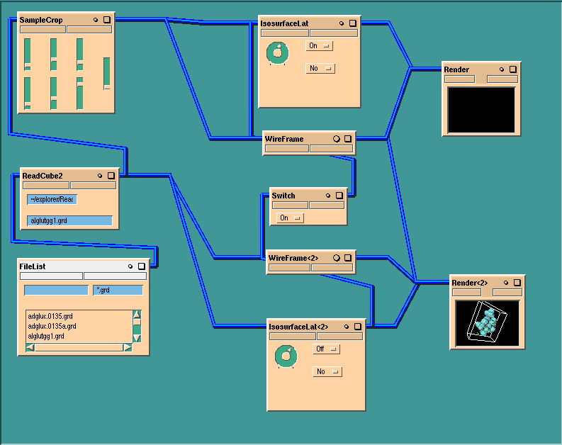
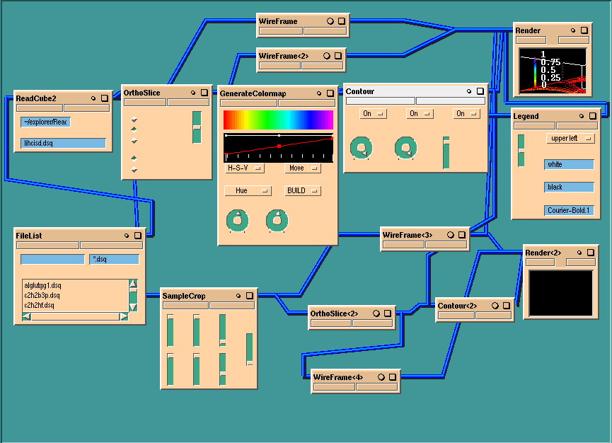
We constructed two explorer maps called DisplayRHO and DisplayContour for the analysis of 3D electron density, the absolute value of gradient, and the Laplacian.
For the visualization of the images one of the various webspace browsers must be installed. We use the SGI version of webspace. If the picture is too dark, switch the headlight on.
Carbon monoxide (3D)
The following surfaces were calculated from the B3P/6-31G(p) electron density. For the references of various methods see paper20 in ECCC2.
The isosurface with Laplacian = 0 a.u. of CO is shown on figure 1. The opening view is of the isosurface of the oxygen end of the molecule. Rotate, the image about 90+ degrees to the right. There are four regions of space where the Laplacian is negative, three of which are visible. Two of the core regions are the 1s electrons of the C and O. The negative core region of the O is hidden by valence shell electrons while the core electrons of the C are visible. The visible region to the right is derived from the valance shell electrons of the O. The negative region to left is derived from the valance shell electrons of the C. The valence shell of the carbon side of the O has a rather distorted shape because of the electron withdrawing effect of the oxygen. The apparent gap between the two negative Laplacian valence regions is not supported by the results of higher level calculations [8]. This gap appears in the HF calculations, and the apparent gap here is certainly the origin of the HF exchange included in the B3P method.
Figure 2 is the green box section of figure 1. The opening front view shows the oxygen at the right side. The 1s shells of the oxygen and carbon are color coded by red and gray, respectively. The position of the BCP is shown by a small green sphere. The outer negative regions are separated by positive regions from the inner negative core regions. Hyperlinks are represented by cube and spheres (red-white-green) at the right side of the object. They show the title, and some future navigation possibility.
The isosurface with Laplacian = -0.3 a.u. of CO is shown on figure 3. These isosurfaces represent the more negative Laplacian concentrations. The lone pair like concentration at the C side is clearly visible. This negative region around the carbon is more extended while the negative region around oxygen is more compact.
Figure 4 is green box section of figure 3.
The isosurfaces for the CF4 were calculated from the MP/6-31G(d) electron density. The isosurface with Laplacian = -0.3 a.u. of CF4 is shown on figure 5. As you rotate the isosurface the four valance shell Laplacian concentration is quite visible around the central C core region in between the C and F nuclei. This tetrahedral concentration pattern of the C valence shell is in perfect agreement with the Lewis scheme. The shell structure of the F atoms are partly visible too, however, the valance shells cover the core regions. The apparent cubic nature of the nucleus and the other distortions is again caused by the low density of the grid points.
Figure 6 shows the isosurface with Laplacian = 0 .3 a.u. of CF4. The positive hole leading to the C nucleus is visible. This figure shows again an interesting shell structure.
Ethylene
The isosurfaces for the ethylene were calculated from the MP/6-31G(d) electron density. The isosurface with Laplacian = 0 au cut in the molecular plane of C2H4 is shown on figure 7. If you rotate this surface to the left you see the chemical bonding in the ethylene. This surface shows again the usual shell structure. What is more interesting, the triangular distortion of the C valence shells is visible on the slightly triangular internal surface of the C valence shell.
Figure 8 shows the isosurface with Laplacian = -0.3 au of ethylene. If you rotate the surface to the right you will see the elliptic double bond region connecting the two carbon atoms, the two carbon core regions and the four sigma type C-H bonds. The picture clearly shows why we speak about double bond in ethylene.
Figure 9 shows the isosurface with Laplacian = -0.8 a.u. of ethylene.
Acknowledgments
The financial support of the Hungarian Research Foundation (OTKA T14975, and T16328) is acknowledged.